这是Lecture 4 – Automatic Differentiation和Lecture 5 – Automatic Differentiation Implementation的学习笔记。
Computational Graph
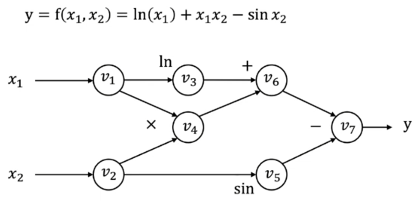
计算图是一个DAG。
Forward evaluation trace
$$
\begin{aligned}
v_1&=x_1=2\\
v_2&=x_2=5\\
v_3&=\ln v1 =\ln 2=0.693\\
v_4&=v1\times v2=10\\
v_5&=\sin v_2=\sin 5 = -0.959\\
v_6&=v_3+v_4=10.693\\
v_7&=v_6-v_5=11.652\\
y&=v_7=11.652
\end{aligned}
$$
Forward mode automatic differentiation(AD)
Define $\overset{\cdot}{v_i}=\frac{\partial v_i}{\partial x_1}$。
$$
\begin{aligned}
\overset{\cdot}{v_1}&=1\quad(v_1=x_1)\\
\overset{\cdot}{v_2}&=0\quad(v_1=x_1)\\
\overset{\cdot}{v_3}&=\frac{\partial \ln v_1}{\partial x_1}=1/v_1 = 0.5\\
\overset{\cdot}{v_4}&=\frac{\partial v_1v_2}{\partial x_1}=\overset{\cdot}{v_1}v_2+\overset{\cdot}{v_2}v_1 = 5\\
\overset{\cdot}{v_5}&=\frac{\partial \sin v_2}{\partial x_1}=\cos v_2\cdot\overset{\cdot}{v_2}=0\\
\overset{\cdot}{v_6}&=\overset{\cdot}{v_3}+\overset{\cdot}{v_4}=5.5\\
\overset{\cdot}{v_7}&=\overset{\cdot}{v_6}-\overset{\cdot}{v_5}=5.5
\end{aligned}
$$
对于映射 $f:\mathbb R^n\to\mathbb R^k$,forward mode AD需要 $n$ 次前向推导才能求出每一个输入的梯度。但是在ML的实际场景下,$n$ 往往很大,而 $k$ 很小。
Reverse mode AD
Define $\bar{v_i}=\frac{\partial y}{\partial v_i}$.
$$
\begin{aligned}
\bar{v_7}&=1\quad(v_7=y)\\
\bar{v_6}&=\frac{\partial y}{\partial v_7}\cdot \frac{\partial v_7}{\partial v_6}=1\cdot \frac{\partial (v_6-v_5)}{\partial v_6}=1\\
\bar{v_5}&=\frac{\partial y}{\partial v_7}\cdot \frac{\partial v_7}{\partial v_5}=1\cdot \frac{\partial (v_6-v_5)}{\partial v_5}=-1\\
\bar{v_4}&=\frac{\partial y}{\partial v_7}\cdot \frac{\partial v_7}{\partial v_6}\cdot \frac{\partial v_6}{\partial v_4}=\bar{v_6}\frac{\partial v_6}{\partial v_4}=1\cdot \frac{\partial (v_3+v_4)}{\partial v_4}=1\\
\bar{v_3}&=\frac{\partial y}{\partial v_7}\cdot \frac{\partial v_7}{\partial v_6}\cdot \frac{\partial v_6}{\partial v_3}=\bar{v_6}\frac{\partial v_6}{\partial v_3}=1\cdot \frac{\partial (v_3+v_4)}{\partial v_4}=1\\
\bar{v_2}&=\bar{v_4}\frac{\partial v_4}{\partial v_2} + \bar{v_5}\frac{\partial v_5}{\partial v_2} = \frac{\partial v_1v_2}{\partial v_2} – \frac{\partial \sin v_2}{\partial v_2} = -0.284\\
\bar{v_1}&=\bar{v_3}\frac{\partial v_3}{\partial v_1} + \bar{v_4}\frac{\partial v_4}{\partial v_1} = \frac{\partial \ln v_1}{\partial v_1}+\frac{\partial v_1v_2}{\partial v_1}=5.5
\end{aligned}
$$
也就是按照反拓扑序求解。不难发现只需要一次反向推导就能求出所有输入的梯度。
Derivation for the multiple pathway case
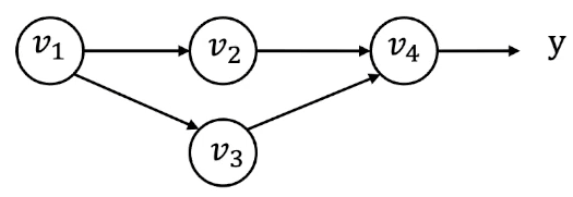
如图所示,$y$ 可以表示为 $y=f(v_2,v_3)$,此时有
$$
\bar{v_1} = \frac{\partial y}{\partial v_1} = \bar{v_2}\frac{\partial v_2}{\partial v_1} + \bar{v_3}\frac{\partial v_3}{\partial v_1}
$$
定义partial adjoint(不知道怎么翻译了,偏导伴随?)$\overline{v_{i\to j}} = \bar{v_j}\frac{\partial v_j}{\partial v_i}$,这里 $i\to j$ 表示在原图中的一条有向边,则有
$$
\bar{v_i} = \sum_{j\in \text{next}(i)} \overline{v_{i\to j}}
$$
这里,partial adjoint伴随原图中的每一条边出现,而任意结点的梯度 $\bar{v_i}$ 就是所有伴随量 $\sum_{j\in \text{next}(i)} \overline{v_{i\to j}}$ 之和。
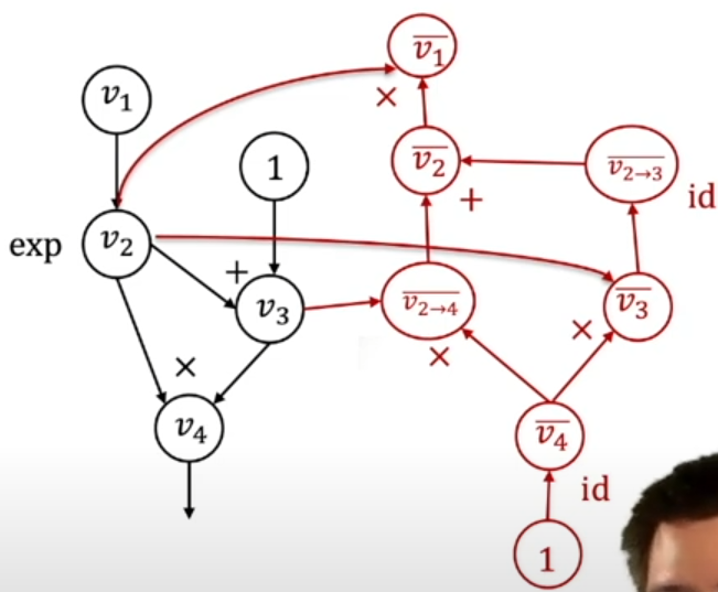
Reverse mode AD by extending computational graph

Reverse mode AD vs backpropagation
- backpropagation只会在forward graph的基础上计算反向传播的梯度
- computational graph是在根据forward graph建立的新图
优势(from GPT)- 自动化管理:计算图框架将复杂的网络结构的梯度计算过程自动化,不需要开发者关注各层之间的依赖关系。这大大简化了模型的实现和调试。
- 高效的内存管理与并行计算:计算图可以优化内存分配,智能地决定哪些部分需要缓存,以及如何有效地执行计算,特别是在多核CPU或GPU上进行并行计算时。
Reverse mode AD on Tensors
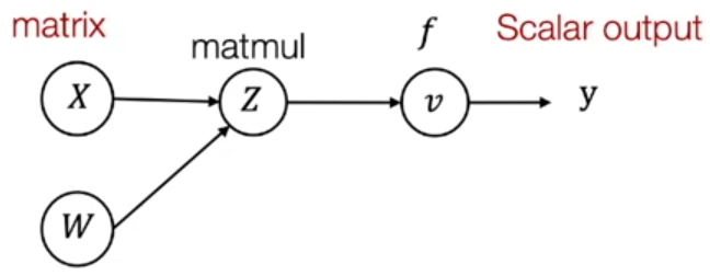
这里 $Z=XW,v=f(Z)=y$,$Z$ 是两个矩阵相乘,也就是 $Z_{ij}=\sum_{k}X_{ik}W_{kj}$。
Define $\bar Z = \pmatrix{
\frac{\partial y}{\partial Z_{1,1}} & \cdots & \frac{\partial y}{\partial Z_{1,n}}\\
\vdots & \ddots & \vdots\\
\frac{\partial y}{\partial Z_{n,1}} & \cdots & \frac{\partial y}{\partial Z_{n,n}}\\
}$
根据矩阵乘法的定义 $Z_{ij}=\sum_{k}X_{ik}W_{kj}$ 可知
$$
\bar{X}_{i,k}=\sum_{j}\frac{\partial Z_{i,j}}{\partial X_{i,k}}\bar{Z}_{i,j} = \sum_{j}W_{k,j}\bar Z_{i,j}
$$
这里 $Z_{i,j} = \sum_{k}X_{ik}W_{kj}$,所以对 $X_{i,k}$ 求偏导后就只剩下了 $W_{k,j}$。于是有
$$
\bar X = \bar Z W^T
$$
Automatic Differentiation Implementation
这一部分是基于dlsys hw1实现的一个简单自动微分系统,采用一个轻量级的needle框架。
该框架的核心定义位于 python/needle/autograd.py,主要由以下几个类构成:
class Op:存储每个结点的运算(正向传播和反向传播)class Value:这是计算图中原图的结点,用于维护每个结点的前驱节点、每个结点是怎么计算的等信息class Tensor(Value):将value封装为tensor,实现和torch.tensor类似的功能
Q1&Q2: ops
这一节主要负责实现自动微分框架中的一些常用运算,也就是 python/needle/ops/ops_mathematic.py 文件中的所有方法。
以文件中已经给出的类为例:
class EWiseMul(TensorOp):
    def compute(self, a: NDArray, b: NDArray):
        return a * b

    def gradient(self, out_grad: Tensor, node: Tensor):
        lhs, rhs = node.inputs
        return out_grad * rhs, out_grad * lhs


def multiply(a, b):
    return EWiseMul()(a, b)
自动微分框架中的每种运算都需要实现两种运算(前向传播和反向传播),这里的 EWiseMul 类维护两个矩阵之间的逐元素相乘,因此前向传播就是
def compute(self, a: NDArray, b: NDArray):
    return a * b
对于反向传播,首先说明 gradient 中的两个参数是什么含义:假设这个运算维护的是 $v_4=v_2* v_3$ 这三个节点之间的运算,根据伴随量的公式可知
$$
\bar{v_2} = \bar{v_4}\frac{\partial v_4}{\partial v_2}=\bar{v_4}v_3, \bar{v_3}=\bar{v_4}\frac{\partial v_4}{\partial v_3}=\bar{v_4}v_2
$$
对应到gradient的参数,这里 out_grad 就是 $\bar{v_4}$,而 node 则是 $v_4$ 在原图中对应的结点,因此 lhs, rhs = node.inputs 就是 $v_2,v_3$(原图中 $v_4$ 的前驱),而gradient返回的则是 $\bar{v_2},\bar{v_3}$。
EWisePow
class EWisePow(TensorOp):
    """Op to element-wise raise a tensor to a power."""

    def compute(self, a: NDArray, b: NDArray) -> NDArray:
        ### BEGIN YOUR SOLUTION
        return array_api.power(a, b)
        ### END YOUR SOLUTION

    def gradient(self, out_grad, node):
        ### BEGIN YOUR SOLUTION
        a, b = node.inputs
        grad_a = out_grad * (b * power(a, b - 1))
        grad_b = out_grad * (power(a, b) * log(a))
        return (grad_a, grad_b)
        ### END YOUR SOLUTION
也就是分别求出 $\frac{\partial a^b}{\partial a}$ 和 $\frac{\partial a^b}{\partial b}$ 的偏导。
PowerScalar
class PowerScalar(TensorOp):
    """Op raise a tensor to an (integer) power."""

    def __init__(self, scalar: int):
        self.scalar = scalar

    def compute(self, a: NDArray) -> NDArray:
        ### BEGIN YOUR SOLUTION
        return a ** self.scalar
        ### END YOUR SOLUTION

    def gradient(self, out_grad, node):
        ### BEGIN YOUR SOLUTION
        return (out_grad * self.scalar * power_scalar(a, self.scalar - 1),)
        ### END YOUR SOLUTION
EWiseDiv
class EWiseDiv(TensorOp):
    """Op to element-wise divide two nodes."""

    def compute(self, a, b):
        ### BEGIN YOUR SOLUTION
        return a / b
        ### END YOUR SOLUTION

    def gradient(self, out_grad, node):
        ### BEGIN YOUR SOLUTION
        a, b = node.inputs
        grad_a = out_grad * power_scalar(b, -1)
        grad_b = -out_grad * power_scalar(b, -2) * a
        return (grad_a, grad_b)
        ### END YOUR SOLUTION
DivScalar
class DivScalar(TensorOp):
    def __init__(self, scalar):
        self.scalar = scalar

    def compute(self, a):
        ### BEGIN YOUR SOLUTION
        return a / self.scalar
        ### END YOUR SOLUTION

    def gradient(self, out_grad, node):
        ### BEGIN YOUR SOLUTION
        return (out_grad / self.scalar,)
        ### END YOUR SOLUTION
Transpose
注意这里的矩阵转置的定义参考hw1中的定义:reverses the order of two axes (axis1, axis2), defaults to the last two axes (1 input, axes – tuple)。
class Transpose(TensorOp):
    def __init__(self, axes: Optional[tuple] = None):
        self.axes = axes

    def compute(self, a):
        ### BEGIN YOUR SOLUTION
        # reverses the order of two axes (axis1, axis2), defaults to the last two axes (1 input, axes - tuple)
        if self.axes:
            return array_api.swapaxes(a, self.axes[0], self.axes[1])
        else:
            return array_api.swapaxes(a, -2, -1)
        ### END YOUR SOLUTION

    def gradient(self, out_grad, node):
        ### BEGIN YOUR SOLUTION
        return (transpose(out_grad, self.axes),)
        ### END YOUR SOLUTION
矩阵转置的梯度怎么理解?注意到矩阵转置并不会改变元素的值,本质上是对元素的一次重新排列,转置的梯度就是转置的逆运算,因此矩阵转置的梯度仍然是矩阵转置。
Reshape
class Reshape(TensorOp):
    def __init__(self, shape):
        self.shape = shape

    def compute(self, a):
        ### BEGIN YOUR SOLUTION
        return array_api.reshape(a, self.shape)
        ### END YOUR SOLUTION

    def gradient(self, out_grad, node):
        ### BEGIN YOUR SOLUTION
        return (reshape(out_grad, node.inputs[0].shape),)
        ### END YOUR SOLUTION
reshape的理解思路和矩阵转置是类似的,reshape本质是重排元素,因此我们只需要将 out_grad 重排为 node.inputs[0] 的维度即可。
BroadcastTo
class BroadcastTo(TensorOp):
    def __init__(self, shape):
        self.shape = shape

    def compute(self, a):
        ### BEGIN YOUR SOLUTION
        return array_api.broadcast_to(a, self.shape)
        ### END YOUR SOLUTION

    def gradient(self, out_grad, node):
        ### BEGIN YOUR SOLUTION
        a = node.inputs[0]
        new_shape = a.shape
        old_shape = out_grad.shape
        if len(old_shape) != len(new_shape):
            new_shape = [1] * (len(old_shape) - len(new_shape))
            new_shape.extend(a.shape)
        dif = [i for i, (x, y) in enumerate(zip(new_shape, old_shape)) if x != y]
        grad_a = summation(out_grad, tuple(dif))
        grad_a = reshape(grad_a, a.shape)
        return grad_a
        ### END YOUR SOLUTION
这是一个比较复杂的类,设计numpy中的广播机制。首先需要先理解numpy中的广播是怎么做的:
- 检查维度:检查两个数组的维度是否相同,如果不同则进入2.
- 维度扩展:维度较少的数组在左侧填1,直到两个数组的维度一致。
- 检查兼容性:两个数组可以广播当且仅当以下条件成立:
- 维度的大小相同。
- 如果维度不同,则其中一个是1。
比如shape分别为
- $(3,3,3),(1)$
- $(2,5),(1,5)$
之类的数组可以广播。
比如shape分别为
- $(2,4,6),(2,2,6)$
- $(5,4),(5)$
之类的数组不能广播。
比较常见的广播的例子就是 $W+C$,这里 $W$ 是一个高维矩阵,而 $C$ 是一个常数,此时numpy就会自动将 $C$ 视作一个shape为 $(1,)$ 的矩阵并广播为 $W$ 的shape。
因此,广播本质上也不会改变元素的值,可以简单地认为广播是沿着某些维度将原本的数组“复制”了几份。
那么广播的梯度怎么计算?一个简单的思路是:广播既然是将元素复制了几份,那么梯度就是将复制品重新聚合到原本的维度。比如 $shape=(3,1)$ 的矩阵广播到 $(3,2)$,那么梯度就是将 $(3,2)$ 的矩阵沿着 axis = 1 求和,将维度重新压回 $(3,1)$。
注意到这个梯度实际上用到了 summation 函数,这个之后会实现。
Summation
class Summation(TensorOp):
    def __init__(self, axes: Optional[tuple] = None):
        self.axes = axes

    def compute(self, a):
        ### BEGIN YOUR SOLUTION
        return array_api.sum(a, axis=self.axes)
        ### END YOUR SOLUTION

    def gradient(self, out_grad, node):
        ### BEGIN YOUR SOLUTION
        a = node.inputs[0]
        old_shape = out_grad.shape
        new_shape = [1] * len(a.shape)
        j = 0
        for i in range(len(a.shape)):
            if j < len(old_shape) and a.shape[i] == old_shape[j]:
                new_shape[i] = old_shape[j]
                j += 1

        grad_a = broadcast_to(reshape(out_grad, new_shape), a.shape)
        return grad_a
        ### END YOUR SOLUTION
求和函数可以认为是广播的逆运算,因此求和的梯度用广播计算(恢复被压缩的维度)。
MatMul
class MatMul(TensorOp):
    def compute(self, a, b):
        ### BEGIN YOUR SOLUTION
        return a @ b
        ### END YOUR SOLUTION

    def gradient(self, out_grad, node):
        ### BEGIN YOUR SOLUTION
        a, b = node.inputs

        grad_a = out_grad @ transpose(b)
        grad_b = transpose(a) @ out_grad
        if grad_a.shape != a.shape:
            broadcast_dims = len(grad_a.shape) - len(a.shape)
            grad_a = summation(grad_a, tuple(range(broadcast_dims)))
        if grad_b.shape != b.shape:
            broadcast_dims = len(grad_b.shape) - len(b.shape)
            grad_b = summation(grad_b, tuple(range(broadcast_dims)))
        assert grad_a.shape == a.shape
        assert grad_b.shape == b.shape
        return grad_a, grad_b
        ### END YOUR SOLUTION
矩阵乘法梯度的推导在Reverse mode AD on Tensors中已经简单介绍过了,简单地说就是对于 $Z=XW$,$\bar X = \bar Z W^T$,而对于 $Z=WX$,$\bar X = W^T\bar Z$。
此外,需要注意我们这里需要实现矩阵乘法的广播,简单地说就是将维度较小的矩阵广播到对应尺寸。
Negate
class Negate(TensorOp):
    def compute(self, a):
        ### BEGIN YOUR SOLUTION
        return -a
        ### END YOUR SOLUTION

    def gradient(self, out_grad, node):
        ### BEGIN YOUR SOLUTION
        return -out_grad
        ### END YOUR SOLUTION
Log
class Log(TensorOp):
    def compute(self, a):
        ### BEGIN YOUR SOLUTION
        return array_api.log(a)
        ### END YOUR SOLUTION

    def gradient(self, out_grad, node):
        ### BEGIN YOUR SOLUTION
        a = node.inputs[0]
        return out_grad / a
        ### END YOUR SOLUTION
Exp
class Exp(TensorOp):
    def compute(self, a):
        ### BEGIN YOUR SOLUTION
        return array_api.exp(a)
        ### END YOUR SOLUTION

    def gradient(self, out_grad, node):
        ### BEGIN YOUR SOLUTION
        a = node.inputs[0]
        return out_grad * exp(a)
        ### END YOUR SOLUTION
ReLU
class ReLU(TensorOp):
    def compute(self, a):
        ### BEGIN YOUR SOLUTION
        b = array_api.copy(a)
        b[b < 0] = 0
        return b
        ### END YOUR SOLUTION

    def gradient(self, out_grad, node):
        ### BEGIN YOUR SOLUTION
        a = node.inputs[0].realize_cached_data()
        a[a < 0] = 0
        a[a > 0] = 1
        return out_grad * a
        ### END YOUR SOLUTION
Question 3: Topological sort
接下来要实现的是计算图的拓扑排序模块,因为计算图的构造是通过反拓扑序实现的。需要实现的 autograd.py 中的 find_topo_sort 和 topo_sort_dfs 这两个函数。
def find_topo_sort(node_list: List[Value]) -> List[Value]:
    """Given a list of nodes, return a topological sort list of nodes ending in them.

    A simple algorithm is to do a post-order DFS traversal on the given nodes,
    going backwards based on input edges. Since a node is added to the ordering
    after all its predecessors are traversed due to post-order DFS, we get a topological
    sort.
    """
    ### BEGIN YOUR SOLUTION
    topo_order = []
    visited = set()
    for node in node_list:
        topo_sort_dfs(node, visited, topo_order)
    return topo_order
    ### END YOUR SOLUTION


def topo_sort_dfs(node, visited, topo_order):
    """Post-order DFS"""
    ### BEGIN YOUR SOLUTION
    if node in visited:
        return
    for i in node.inputs:
        topo_sort_dfs(i, visited, topo_order)
    topo_order.append(node)
    visited.add(node)
### END YOUR SOLUTION实际上注释中已经说明了,直接按照后序遍历原图就可以求出原图所有结点的拓扑排列。node_list 中的元素就是原图网络中的所有汇点。
Question 4: Implementing reverse mode differentiation
接下来要实现的就是核心的reverse mode AD模块,也就是计算图的反向传播系统。需要实现的 autograd.py 中的 compute_gradient_of_variables 函数。
这一部分代码可以参考Reverse mode AD by extending computational graph章节中的伪代码。
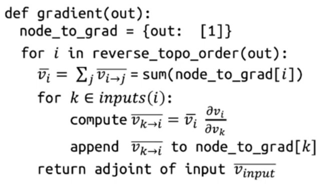
伪代码中的 node_to_grad,也就是下面的 node_to_output_grads_list,存储了整个计算图。node_to_grad[k] 是一个列表,存储了所有 $\overline{v_{k\to i}}$(可以理解为原图中反向边的伴随量)。
def compute_gradient_of_variables(output_tensor, out_grad):
    """Take gradient of output node with respect to each node in node_list.

    Store the computed result in the grad field of each Variable.
    """
    # a map from node to a list of gradient contributions from each output node
    node_to_output_grads_list: Dict[Tensor, List[Tensor]] = {}
    # Special note on initializing gradient of
    # We are really taking a derivative of the scalar reduce_sum(output_node)
    # instead of the vector output_node. But this is the common case for loss function.
    node_to_output_grads_list[output_tensor] = [out_grad]

    # Traverse graph in reverse topological order given the output_node that we are taking gradient wrt.
    reverse_topo_order = list(reversed(find_topo_sort([output_tensor])))

    ### BEGIN YOUR SOLUTION
    for i in reverse_topo_order:
        v_i = sum_node_list(node_to_output_grads_list[i])
        i.grad = v_i
        if i.is_leaf():
            continue
        v_kis = i.op.gradient_as_tuple(v_i, i)
        for j, k in enumerate(i.inputs):
            v_ki = v_kis[j]
            if k not in node_to_output_grads_list:
                node_to_output_grads_list[k] = []
            node_to_output_grads_list[k].append(v_ki)
    ### END YOUR SOLUTION
这个函数会被 Tensor 的 backward 方法调用:
def backward(self, out_grad=None):
    out_grad = (
        out_grad
        if out_grad
        else init.ones(*self.shape, dtype=self.dtype, device=self.device)
    )
    compute_gradient_of_variables(self, out_grad)
因此,该框架和pytorch基本一致,只需要 loss.backward() 就会自动建立计算图并进行反向传播。
Question 5&6
这两部分和hw0基本是一样的,只不过将softmax regression替换为了本节中写的needle框架中的api。
def parse_mnist(image_filesname, label_filename):
    """Read an images and labels file in MNIST format.  See this page:
    http://yann.lecun.com/exdb/mnist/ for a description of the file format.

    Args:
        image_filename (str): name of gzipped images file in MNIST format
        label_filename (str): name of gzipped labels file in MNIST format

    Returns:
        Tuple (X,y):
            X (numpy.ndarray[np.float32]): 2D numpy array containing the loaded
                data.  The dimensionality of the data should be
                (num_examples x input_dim) where 'input_dim' is the full
                dimension of the data, e.g., since MNIST images are 28x28, it
                will be 784.  Values should be of type np.float32, and the data
                should be normalized to have a minimum value of 0.0 and a
                maximum value of 1.0.

            y (numpy.ndarray[dypte=np.int8]): 1D numpy array containing the
                labels of the examples.  Values should be of type np.int8 and
                for MNIST will contain the values 0-9.
    """
    ### BEGIN YOUR SOLUTION
    with gzip.open(image_filesname, 'rb') as f:
        data = f.read()
        num_images = int.from_bytes(data[4:8], byteorder='big')
        num_rows = int.from_bytes(data[8:12], byteorder='big')
        num_cols = int.from_bytes(data[12:16], byteorder='big')
        images = np.frombuffer(data[16:], dtype=np.uint8).reshape(num_images, num_rows * num_cols)
        images = images.astype(np.float32) / 255.0

    with gzip.open(label_filename, 'rb') as f:
        data = f.read()
        labels = np.frombuffer(data[8:], dtype=np.uint8)

    return images, labels
    ### END YOUR SOLUTION


def softmax_loss(Z, y_one_hot):
    """Return softmax loss.  Note that for the purposes of this assignment,
    you don't need to worry about "nicely" scaling the numerical properties
    of the log-sum-exp computation, but can just compute this directly.

    Args:
        Z (ndl.Tensor[np.float32]): 2D Tensor of shape
            (batch_size, num_classes), containing the logit predictions for
            each class.
        y (ndl.Tensor[np.int8]): 2D Tensor of shape (batch_size, num_classes)
            containing a 1 at the index of the true label of each example and
            zeros elsewhere.

    Returns:
        Average softmax loss over the sample. (ndl.Tensor[np.float32])
    """
    ### BEGIN YOUR SOLUTION
    exp_Z = ndl.ops.exp(Z)
    sum_Z = ndl.ops.summation(exp_Z, (1,))
    sum_Z = ndl.ops.reshape(sum_Z, (sum_Z.shape[0], 1))
    sum_Z = ndl.ops.broadcast_to(sum_Z, exp_Z.shape)
    softmax_probs = ndl.ops.divide(exp_Z, sum_Z)

    probs = ndl.ops.multiply(softmax_probs, y_one_hot)
    probs = ndl.ops.summation(probs, (1,))
    probs = -ndl.ops.log(probs)
    loss = ndl.ops.summation(probs)
    loss = loss / Z.shape[0]

    return loss
    ### END YOUR SOLUTION


def nn_epoch(X, y, W1, W2, lr=0.1, batch=100):
    """Run a single epoch of SGD for a two-layer neural network defined by the
    weights W1 and W2 (with no bias terms):
        logits = ReLU(X * W1) * W1
    The function should use the step size lr, and the specified batch size (and
    again, without randomizing the order of X).

    Args:
        X (np.ndarray[np.float32]): 2D input array of size
            (num_examples x input_dim).
        y (np.ndarray[np.uint8]): 1D class label array of size (num_examples,)
        W1 (ndl.Tensor[np.float32]): 2D array of first layer weights, of shape
            (input_dim, hidden_dim)
        W2 (ndl.Tensor[np.float32]): 2D array of second layer weights, of shape
            (hidden_dim, num_classes)
        lr (float): step size (learning rate) for SGD
        batch (int): size of SGD mini-batch

    Returns:
        Tuple: (W1, W2)
            W1: ndl.Tensor[np.float32]
            W2: ndl.Tensor[np.float32]
    """

    ### BEGIN YOUR SOLUTION
    for i in range(X.shape[0] // batch):
        batch_X = X[i * batch: (i + 1) * batch]
        batch_y = y[i * batch: (i + 1) * batch]
        batch_X = ndl.Tensor(batch_X)

        Z = ndl.ops.relu(batch_X @ W1) @ W2
        y_one_hot = np.zeros(Z.shape)
        y_one_hot[np.arange(batch_y.shape[0]), batch_y] = 1
        y_one_hot = ndl.Tensor(y_one_hot, dtype=np.uint8)

        loss = softmax_loss(Z, y_one_hot)
        loss.backward()

        W1 = (W1 - lr * W1.grad).detach()
        W2 = (W2 - lr * W2.grad).detach()
    return W1, W2
    ### END YOUR SOLUTION
不难发现 nn_epoch 这个函数几乎就是pytorch框架的写法了。需要注意的是 W1, W2 在梯度更新后需要重新建立计算图,这里可以调用detach方法以清空原有的梯度信息(因为我们并没有实现torch中的optimizer,只是手写了一个最简单的SGD)。